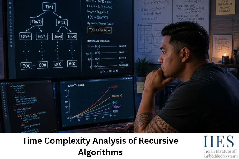
Understanding Time Complexity in DSA
Time complexity in DSA describes how the number of operations performed by an algorithm grows with the input size (n). It is commonly expressed using asymptotic notations such as Big O notation.
Some common time complexities are:
- O(1) — Constant time
- O(log n) — Logarithmic time
- O(n) — Linear time
- O(n log n) — Linearithmic time
- O(n2) — Quadratic time
For recursive algorithms, we often use recurrence relations to represent the work performed by a function and its recursive calls.
Time Complexity Analysis of a Loop
Consider the following C-style loop:
for (i = 5; i <= n; i = i * i) {
    printf("IIES");
}
In this loop, the variable i is squared in every iteration instead of being incremented by a constant value.
Let’s examine the sequence of values:
- First iteration: i = 5
- Second iteration: i = 25
- Third iteration: i = 625
- Fourth iteration: i = 390625
The loop stops when i becomes greater than n.
Deriving the Time Complexity
After repeated squaring, the values of i follow this pattern:
i = 5, 52, 54, 58, …
After k squaring operations, the value is:
i = 52k
The loop condition is:
52k ≤ n
Taking logarithms with base 5:
2k ≤ log5 n
Taking logarithms with base 2 again:
k ≤ log2(log5 n)
Therefore, the number of iterations grows approximately as:
O(log log n)
This is a double logarithmic time complexity, which grows very slowly as the input size increases.
Example: When n = 25
The loop executes with i = 5 and i = 25. After that, i becomes 625, and the condition fails.
Therefore, the printf() statement executes 2 times.
Example: When n = 125
The sequence is:
5 → 25 → 625
The loop executes for i = 5 and i = 25. When i becomes 625, the loop terminates.
Therefore, the printf() statement executes 2 times.
For n ≥ 5, the exact number of iterations can be expressed as:
⌊log2(log5 n)⌋ + 1
This formula accounts for the initial iteration at i = 5, assuming exact arithmetic and the stated loop condition.

Analysing Time for Recursive Programs
What Is a Recursive Function?
A recursive function is a function that calls itself to solve a smaller version of the same problem. Every correctly designed recursive function needs a base case to stop the recursive calls.
Consider the following C function:
int fun(int n) {
    if (n <= 1)
        return 1;
    else
        return fun(n / 2) + n;
}
In this example:
- Base case: If
n <= 1, the function returns 1. - Recursive case: If
n > 1, the function calls fun(n / 2). - Additional operation: The current value of
n is added to the returned result.
For example, when n = 8, the recursive calls follow this sequence:
fun(8) → fun(4) → fun(2) → fun(1)
The base case is reached when the argument becomes 1.
What Is a Recurrence Relation in Algorithms?
A recurrence relation is a mathematical equation that describes the running time of a recursive algorithm in terms of the running time for smaller inputs.
To analyze a recursive function, we represent its running time using T(n).
For the function above, each call performs constant-time work apart from the recursive call. The recurrence relation is:
T(n) = T(n/2) + Θ(1)
Our actual example includes the operation fun(n / 2) + n. The + n in the C statement represents an arithmetic value being added; it does not mean the program performs n separate operations. Counting the work needed for the addition and other constant-time operations still gives the same recurrence, so the time complexity of this particular function is O(log n).
Important: The recurrence relation must represent the number of operations performed, not simply copy the mathematical value returned by the function.
Methods for Solving Recurrence Relations
Several techniques are used for solving recurrence relations and finding the time complexity of recursive algorithms.
- Substitution method: Repeatedly expands the recurrence to identify a pattern and derive a bound.
- Recursion tree method: Represents recursive calls as a tree and calculates the work at each level.
- Master theorem: Provides solutions for certain divide-and-conquer recurrences.
- Change of variables method: Transforms a recurrence into a more familiar form.
- Discrete mathematics techniques: Use mathematical reasoning, summations, and related methods to solve recurrence equations.
Each technique has its own advantages and limitations. The best method depends on the form of the recurrence relation.

Solving Recurrence Relations Using the Substitution Method
The substitution method in recurrence relations solves a recurrence by repeatedly expanding it, observing the resulting pattern, and determining the final complexity.
Consider the following recurrence:
T(n) = T(n/2) + n
This is a different recurrence from the earlier C function. Here, the term +n represents linear work performed at each recursive level.
Assume the base condition is T(1) = 1.
Step 1: Expand the Recurrence
Start with:
T(n) = T(n/2) + n
Substitute T(n/2) into the equation:
T(n) = T(n/4) + n/2 + n
Expand again:
T(n) = T(n/8) + n/4 + n/2 + n
After repeating this process k times:
T(n) = T(n/2k) + Σj=0k−1 (n / 2j)
This is the iterative expansion of the recurrence relation.
Step 2: Identify the Base Case
The recursion stops when:
n / 2k = 1
Therefore:
2k = n
Taking logarithms:
k = log2 n
The number of recursive levels is approximately log2 n.
Step 3: Apply the Geometric Progression Formula
The expanded recurrence contains the series:
n + n/2 + n/4 + n/8 + …
This is a geometric progression (GP) with first term a = n and common ratio r = 1/2.
For a finite geometric progression where r ≠ 1:
Sk = a(1 − rk) / (1 − r)
Substituting a = n and r = 1/2:
Sk = n(1 − (1/2)k) / (1 − 1/2)
Simplifying:
Sk = 2n(1 − 1/2k)
Since 2k = n when n is a power of two:
Sk = 2n − 2
Including the base-case cost T(1) = 1:
T(n) = 1 + 2n − 2
Therefore:
T(n) = 2n − 1
For powers of two under the stated base-case assumption, this is the exact result. For general input sizes, the same asymptotic bound applies.
Hence, the final time complexity is:
T(n) = Θ(n)
The substitution method helps us understand how the work accumulates across recursive calls and determine the asymptotic time complexity.
Difference Between T(n) = T(n/2) + n and T(n) = T(n/2) + 1
These recurrence relations look similar, but their time complexities are different.
| Recurrence relation | Work at each level | Time complexity |
| T(n) = T(n/2) + n | Decreases geometrically | Θ(n) |
| T(n) = T(n/2) + 1 | Constant work | Θ(log n) |
In the first recurrence, the total work is a geometric series dominated by its first term. In the second recurrence, each level contributes constant work, and there are approximately log2 n levels.
Understanding this difference is essential when analysing recursive functions in C and other programming languages.
When Should You Use the Substitution Method?
The substitution method is useful when you can repeatedly expand a recurrence and recognize a pattern. It works well for many basic recurrence relations used in DSA.
However, complicated recurrences may be easier to solve with a recursion tree, Master theorem, or another mathematical technique. The Master theorem, in particular, applies only to certain recurrence forms and should not be used indiscriminately.