What Is Dijkstra’s Algorithm?
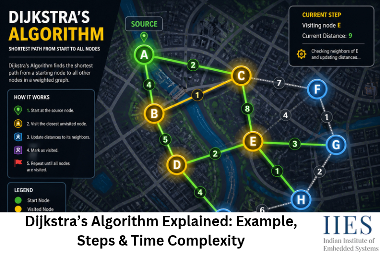
Dijkstra’s algorithm is a greedy algorithm that finds the shortest path from a given source vertex to every other vertex in a weighted graph, provided all edge weights are non-negative.
A weighted graph is a graph in which each edge has an associated value called a weight. This weight may represent distance, cost, time, or another measurable quantity.
For example, in a road network:
- Vertices represent cities.
- Edges represent roads connecting cities.
- Edge weights represent distances between cities.
Dijkstra’s algorithm determines the minimum total distance required to travel from a selected source city to other cities. This process is also known as Dijkstra’s shortest path algorithm in graph theory.
Why Is It Called a Greedy Algorithm?
A greedy algorithm makes the best available choice at each step, hoping to build an optimal solution.
Dijkstra’s algorithm follows this strategy by repeatedly selecting the unvisited vertex with the smallest known distance from the source.
Once a vertex with the smallest tentative distance is selected, its shortest distance is finalized, provided all edge weights are non-negative.
The algorithm then checks whether travelling through that vertex can produce shorter paths to its neighboring vertices. This approach demonstrates how a greedy algorithm in data structures works when solving a shortest-path problem.

Step-by-Step Execution of Dijkstra’s Algorithm
Consider the following weighted undirected graph.
For reference, the edges of this graph (as used in the steps below) are:
| Edge | Weight |
| A – B | 4 |
| A – C | 1 |
| C – B | 2 |
| C – D | 5 |
| B – D | 1 |
| B – E | 7 |
| D – E | 3 |
Our objective is to find the shortest distance from source vertex A to every other vertex using Dijkstra’s algorithm step by step.
Step 1: Initialization
Initially assign a distance of 0 to the source vertex A and infinity to all other vertices because their shortest distances are not yet known.
| Vertex | Distance from A |
| A | 0 |
| B | ∞ |
| C | ∞ |
| D | ∞ |
| E | ∞ |
Step 2: Select vertex A
A has the smallest distance, which is 0.
Its neighbors are B and C.
- Distance to B = 0 + 4 = 4
- Distance to C = 0 + 1 = 1
Mark A as visited.
| Vertex | Distance from A |
| A | 0 |
| B | 4 |
| C | 1 |
| D | ∞ |
| E | ∞ |
Step 3: Select vertex C
Among the unvisited vertices, C has the smallest distance of 1.
Check its neighbors:
- Through C, distance to B = 1 + 2 = 3. This is shorter than 4, so update B to 3.
- Through C, distance to D = 1 + 5 = 6. Update D to 6.
Mark C as visited.
| Vertex | Distance from A |
| A | 0 |
| B | 3 |
| C | 1 |
| D | 6 |
| E | ∞ |
Step 4: Select vertex B
B has the smallest unvisited distance of 3.
Check its neighbors and update the distances:
- Through B, distance to D = 3 + 1 = 4. This is shorter than 6, so update D to 4.
- Through B, distance to E = 3 + 7 = 10. Update E to 10.
Mark B as visited.
| Vertex | Distance from A |
| A | 0 |
| B | 3 |
| C | 1 |
| D | 4 |
| E | 10 |
Step 5: Select vertex D
D has the smallest unvisited distance of 4.
Check its neighbor E:
- Through D, distance to E = 4 + 3 = 7.
- The previous distance to E was 10, so update it to 7.
Mark D as visited.
| Vertex | Distance from A |
| A | 0 |
| B | 3 |
| C | 1 |
| D | 4 |
| E | 7 |
Step 6: Select vertex E
E is the remaining unvisited vertex, with distance 7.
Mark E as visited. The algorithm is complete as all vertices have been covered.
| Vertex | Distance from A |
| A | 0 |
| B | 3 |
| C | 1 |
| D | 4 |
| E | 7 |
Final Shortest Distances
The following table shows the final result of finding the shortest path using Dijkstra’s algorithm.
| Destination | Shortest path from A | Total distance |
| A | A | 0 |
| B | A → C → B | 3 |
| C | A → C | 1 |
| D | A → C → B → D | 4 |
| E | A → C → B → D → E | 7 |
Notice that the direct path from A to B has a cost of 4. However, travelling through C gives a total cost of 1 + 2 = 3, which is shorter. This demonstrates why checking alternative paths is essential in a shortest path algorithm in a weighted graph.
Pseudocode for Dijkstra’s Algorithm
The following Dijkstra’s algorithm pseudocode explains the basic steps involved in finding the shortest distances from a source vertex.
Dijkstra(Graph, source)

1. Set the source vertex distance to 0.
2. Set all other vertex distances to INF.
3. Mark all vertices as unvisited.
4. Repeat until no unvisited vertex with a finite distance remains:
     a. Select the unvisited vertex u with the smallest distance.
     b. If no reachable unvisited vertex exists, stop.
     c. Mark u as visited.
     d. For each unvisited neighbor v of u:
          If distance[u] + weight(u, v) < distance[v], update:
               distance[v] = distance[u] + weight(u, v)
5. Return the distance[] array.
This pseudocode illustrates the fundamental Dijkstra’s algorithm implementation logic used in graph-based shortest-path problems.
Time Complexity of Dijkstra’s Algorithm
The Dijkstra’s algorithm time complexity depends on the data structures used to implement the algorithm.
a. Using an adjacency matrix
When the algorithm searches all vertices to find the smallest unvisited distance, the time complexity is:
O(V2)
Here, V represents the number of vertices.
b. Using an adjacency list and a binary min-heap
A priority queue helps select the vertex with the smallest tentative distance efficiently.
The typical time complexity is:
O((V + E) log V)
Here:
- V = number of vertices
- E = number of edges
For dense graphs or small graphs, an adjacency matrix may be a convenient implementation. For sparse graphs, an adjacency list with a min-heap is often more efficient.
Understanding these complexities is important when comparing different shortest path algorithms in data structures, particularly when working with large graphs.

Applications of Dijkstra’s Algorithm
Dijkstra’s algorithm has several practical applications. These Dijkstra’s algorithm applications demonstrate how shortest-path calculations are used in real-world systems.
1. GPS and route planning
Navigation systems can use shortest-path algorithms to determine routes based on distance or travel cost. Real navigation systems may use additional techniques and changing traffic information.
2. Computer networks
Routing protocols such as OSPF use Dijkstra’s shortest-path algorithm to calculate shortest-path trees from a router.
Robots can use shortest-path techniques to find routes through a map or grid, where edge weights represent movement costs.
4. Transportation systems
The algorithm can help determine low-cost routes through networks of roads, railway connections, or other transport links.
5. Game development
Games can use shortest-path algorithms to help characters navigate maps and reach destinations.
Limitations of Dijkstra’s Algorithm
Although Dijkstra’s algorithm is useful, it has some limitations:
- It assumes that edge weights are non-negative.
- It does not correctly solve the general shortest-path problem when negative-weight edges are present.
- A disconnected graph may contain vertices that cannot be reached from the source.
- A simple adjacency-matrix implementation may be inefficient for very large, sparse graphs.
- When negative edge weights must be supported, the Bellman–Ford algorithm is a common alternative.
This is an important consideration when understanding Dijkstra’s algorithm vs Bellman-Ford, as both algorithms solve shortest-path problems but have different capabilities.
Dijkstra’s algorithm starts by assigning a distance of 0 to the source vertex and infinity to all other vertices. It then selects the unvisited vertex with the smallest distance, updates the distances of its neighboring vertices, and marks the selected vertex as visited. This process continues until all reachable vertices have been processed.
Practice Question
Consider a weighted graph with vertices A, B, C, and D, and edges:
Consider A as the source vertex, calculate the shortest distance to each vertex. Show the tentative distances after every iteration and identify the final shortest paths.
This practice question helps learners understand how to find the shortest path using Dijkstra’s algorithm and apply the algorithm to a different weighted graph.
Conclusion
Dijkstra’s algorithm is an important graph algorithm that demonstrates how a greedy strategy can solve a shortest-path problem.
By repeatedly selecting the unvisited vertex with the smallest tentative distance and relaxing its neighboring edges, the algorithm determines the shortest distances from a source to all reachable vertices.
Understanding this algorithm builds a strong foundation for studying graph traversal, greedy algorithms, network routing, and other advanced Data Structures and Algorithms topics.
Dijkstra’s algorithm finds shortest paths in weighted directed and undirected graphs with non-negative edge weights by making the best available distance choice at each step.
Learning Dijkstra’s shortest path algorithm, its implementation, time complexity, and practical applications provides a strong foundation for understanding graph algorithms and solving advanced programming problems.